library(readr)
library(here)      ### for robust relative file paths
library(dplyr)
library(tidyr)
library(forcats)   ### tools for working with factors (e.g., reordering)
library(janitor)   ### clean column names

### Visualization
library(ggplot2)

### Interactive output
library(plotly)
library(DT)
library(leaflet)Data Visualization
Load packages
Load the data
# read in data from the data directory after manually downloading data
#| output: false
delta_visits_raw <- read_csv(here("Data/Socioecological_monitoring_data.csv"))
Rows: 55 Columns: 13
── Column specification ────────────────────────────────────────────────────────
Delimiter: ","
chr (4): EcoRestore_approximate_location, Reach, Time_of_Day, notes
dbl (8): Latitude, Longitude, sm_boat, med_boat, lrg_boat, bank_angler, sci...
date (1): Date
ℹ Use `spec()` to retrieve the full column specification for this data.
ℹ Specify the column types or set `show_col_types = FALSE` to quiet this message.### Check out column names
colnames(delta_visits_raw) [1] "EcoRestore_approximate_location" "Reach"
[3] "Latitude" "Longitude"
[5] "Date" "Time_of_Day"
[7] "sm_boat" "med_boat"
[9] "lrg_boat" "bank_angler"
[11] "scientist" "cars"
[13] "notes" ### Peek at each column and class
glimpse(delta_visits_raw)Rows: 55
Columns: 13
$ EcoRestore_approximate_location <chr> "Decker Island", "Decker Island", "Dec…
$ Reach <chr> "Brannan to Decker Island", "Decker Is…
$ Latitude <dbl> 38.10587, 38.10587, 38.08456, 38.08456…
$ Longitude <dbl> -121.7064, -121.7064, -121.7204, -121.…
$ Date <date> 2017-07-07, 2017-07-07, 2017-07-07, 2…
$ Time_of_Day <chr> "unknown", "unknown", "unknown", "unkn…
$ sm_boat <dbl> 0, 0, 0, 0, 2, 0, 0, 7, 1, 0, 0, 0, 0,…
$ med_boat <dbl> 2, 4, 0, 1, 10, 0, 0, 1, 2, 0, 1, 6, 1…
$ lrg_boat <dbl> 0, 0, 0, 0, 1, 0, 0, 0, 0, 0, 0, 0, 0,…
$ bank_angler <dbl> 1, 3, 0, 0, 0, 0, 0, 0, 2, 0, 0, 5, 0,…
$ scientist <dbl> 0, 0, 0, 0, 0, 0, 0, 0, 0, 0, 0, 0, 0,…
$ cars <dbl> 0, 0, 0, 0, 0, 0, 0, 0, 0, 0, 0, 0, 0,…
$ notes <chr> "no notes", "no notes", "Nobody or tra…### From when to when
range(delta_visits_raw$Date)[1] "2017-07-07" "2018-03-13"### Which time of day?
unique(delta_visits_raw$Time_of_Day)[1] "unknown" "morning"colnames(delta_visits_raw)[1:6][1] "EcoRestore_approximate_location" "Reach"
[3] "Latitude" "Longitude"
[5] "Date" "Time_of_Day" delta_visits <- delta_visits_raw %>%
janitor::clean_names()
colnames(delta_visits)[1:6][1] "eco_restore_approximate_location" "reach"
[3] "latitude" "longitude"
[5] "date" "time_of_day" visits_long <- delta_visits %>%
tidyr::pivot_longer(
cols = c(sm_boat, med_boat, lrg_boat, bank_angler, scientist, cars),
names_to = "visitor_type",
values_to = "quantity"
) %>%
### shorten the long name:
dplyr::rename(restore_loc = eco_restore_approximate_location) %>%
### drop the notes column:
dplyr::select(-notes)
glimpse(visits_long)Rows: 330
Columns: 8
$ restore_loc <chr> "Decker Island", "Decker Island", "Decker Island", "Decke…
$ reach <chr> "Brannan to Decker Island", "Brannan to Decker Island", "…
$ latitude <dbl> 38.10587, 38.10587, 38.10587, 38.10587, 38.10587, 38.1058…
$ longitude <dbl> -121.7064, -121.7064, -121.7064, -121.7064, -121.7064, -1…
$ date <date> 2017-07-07, 2017-07-07, 2017-07-07, 2017-07-07, 2017-07-…
$ time_of_day <chr> "unknown", "unknown", "unknown", "unknown", "unknown", "u…
$ visitor_type <chr> "sm_boat", "med_boat", "lrg_boat", "bank_angler", "scient…
$ quantity <dbl> 0, 2, 0, 1, 0, 0, 0, 4, 0, 3, 0, 0, 0, 0, 0, 0, 0, 0, 0, …daily_visits_loc <- visits_long %>%
group_by(restore_loc, date, visitor_type) %>%
summarize(daily_visits = sum(quantity), .groups = "drop")Data viz!
daily_visits_loc %>%
    filter(daily_visits < 30,
    visitor_type %in% c("sm_boat", "med_boat", "lrg_boat")) %>%
    ggplot(aes(x = visitor_type, y = daily_visits)) +
    geom_col(aes(fill = visitor_type))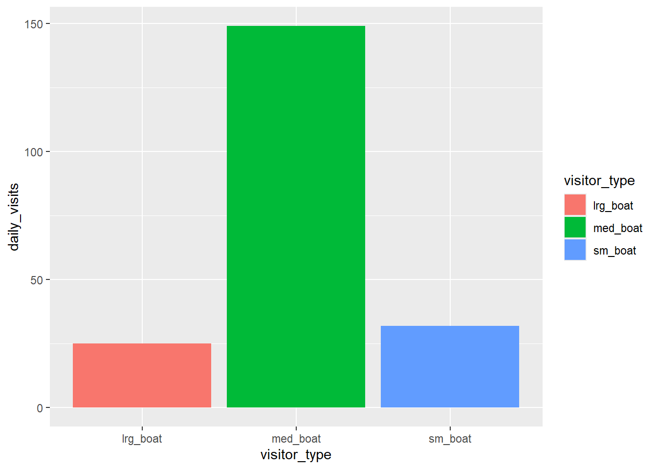
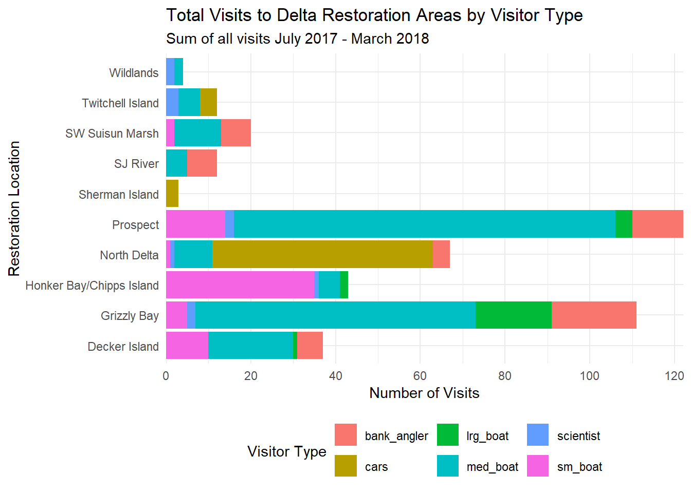
ggplot(data = daily_visits_loc,
       aes(y = restore_loc, x = daily_visits, fill = visitor_type)) +
  geom_col() +
  labs(x = "Number of Visits",
       y = "Restoration Location",
       fill = "Visitor Type",
       title = "Total Visits to Delta Restoration Areas by Visitor Type",
       subtitle = "Sum of all visits July 2017 - March 2018") +
  scale_x_continuous(breaks = seq(0, 120, 20), expand = c(0, 0)) +
  theme_minimal() +
  theme(
    legend.position = "bottom",
    axis.ticks.y = element_blank()
  )
### Save the plot

#ggsave("Plots/visit_restore_site_delta.jpg", width = 12, height = 6, units = "in")
daily_visits_totals <- daily_visits_loc %>%
group_by(restore_loc) %>%
mutate(total = sum(daily_visits)) %>%
ungroup() %>%
mutate(restore_loc = fct_reorder(restore_loc, desc(total)))
unique(daily_visits_totals$restore_loc) [1] Decker Island Grizzly Bay Honker Bay/Chipps Island
[4] North Delta Prospect SJ River
[7] SW Suisun Marsh Sherman Island Twitchell Island
[10] Wildlands
10 Levels: Prospect Grizzly Bay North Delta ... Sherman Islandfacet_plot <- ggplot(data = daily_visits_totals,
aes(x = visitor_type, y = daily_visits,
fill = visitor_type)) +
geom_col() +
facet_wrap(~restore_loc,
scales = "free_y", #unique ranges for the y scale
ncol = 5,
nrow = 2) +
scale_fill_viridis_d() +
labs(x = "Type of visitor",
y = "Number of Visits",
title = "Total Number of Visits to Delta Restoration Areas",
subtitle = "Sum of all visits during study period") +
theme_bw() +
theme(legend.position = "bottom",
axis.ticks.x = element_blank(),
axis.text.x = element_blank())
facet_plot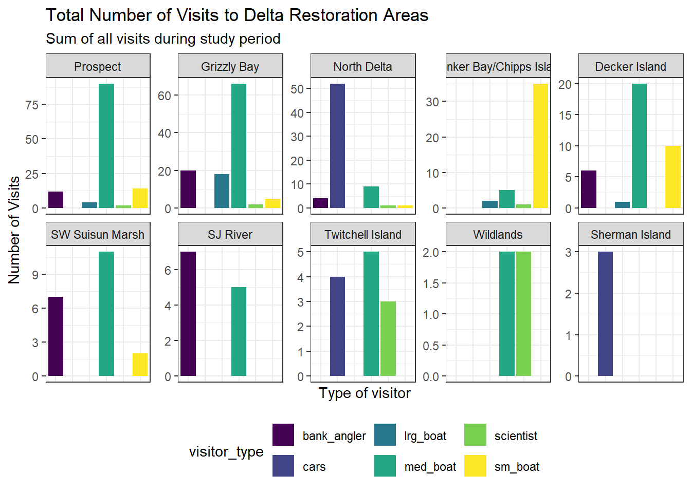
## Interactive plots!!

ggplotly(facet_plot, tooltip = c('x', 'y'))
Show an interactive table
datatable(delta_visits)Show interactive map
Interactive Map
restoration_sites <- delta_visits_raw %>%
  janitor::clean_names() %>%
  distinct(restore_loc = eco_restore_approximate_location,
           latitude, longitude) %>%
  drop_na(latitude, longitude)

leaflet(restoration_sites) %>%
  addTiles() %>%
  addMarkers(
    lng   = ~longitude,
    lat   = ~latitude,
    popup = ~restore_loc
  )